tttplots - a perl program to create time-to-target plots


Renata M. Aiex1, Mauricio G. C. Resende2, and Celso C. Ribeiro3

1Catholic U. of Rio de Janeiro, Brazil.
2AT&T Labs Research, Florham Park, New Jersey, USA.
3U. Federal Fluminense, Niterói, Rio de Janeiro, Brazil.

October 2005

Click here to download the paper [PDF: 249 Kb].


INTRODUCTION

This web page describes a perl program to plot time-to-target (ttt) plots for measured CPU times that are assumed to fit a shifted exponential distribution
.  This is often the case in local search based heuristics for combinatorial optimization, such as simulated annealing, genetic algorithms, iterated local search, tabu search, WalkSAT, and GRASP (Aiex, Resende, and Ribeiro, 2002; Battiti and Tecchiolli, 1992; Dodd, 1990; Ten Eikelder et al., 1996; Osborne and Gillett, 1991; Selman, Kautz, and Cohen, 1994; Taillard, 1991; Verhoeven and Aarts, 1995).  We first discuss how ttt plots are generated, following closely Aiex, Resende, and Ribeiro (2002).  Then, we describe the perl program tttplots.pl.

TTT PLOTS

The hypothesis here is that CPU times fit a two parameter, or shifted, exponential distribution. For a given problem instance, we measure the CPU time to find an objective function value at least as good as a given target value.  The heuristic is run n  times on the fixed instance and using the given target solution. For each of the n runs, the random number generator is initialized with a distinct seed and therefore the runs are assumed to be independent. To compare the empirical and the theoretical distributions, we follow a standard graphical methodology for data analysis (Chambers et al., 1983).  This methodology produces the ttt plots. In the remainder of this section we describe this methodology.

For each instance/target pair, the running times are sorted in increasing order. We associate with the i-th sorted running time t(i) a probability p(i) = (i-1/2)/n, and plot the points z(i) = [t(i),p(i)], for i = 1, ...,n.  Figure 1 illustrates this cumulative probability distribution plot for a instance/target pair for a GRASP.  In this figure, we see that the probability of the heuristic finding a solution at least as good as the target value in at most 2 seconds is about 50%, in st most 4 seconds is about 80%, and in at most 6 seconds is about 90%.

Cumulative probability distribution
Figure 1 - Cumulative probability distribution


The plot in Figure 1 appears to fit a shifted exponential distribution.  We would like to estimate the parameters of the two-parameter exponential distribution.  To do this, we first draw the theoretical quantile-quantile plot (or Q-Q plot) for the data. To describe Q-Q plots, we recall that the cumulative distribution function for the two-parameter exponential distribution is given by F(t) = 1 - exp[-(t-M)/L], where L is the mean of the distribution data (and also indicates the spread of the data) and M is the shift of the distribution with respect to the ordinate axis.

For each value p(i), i=1, ..., n, we associate a p(i)-quantile Qt(p(i)) of the theoretical distribution. For each p(i)-quantile we have, by definition, that F((Qt(p(i))) = p(i). Hence, Qt(p(i)) = F--1(p(i)) and therefore, for the two-parameter exponential distribution, we have Qt(p(i)) = -L ln(1 - p(i)) + M. The quantiles of the data of an empirical distribution are simply the (sorted) raw data.

A theoretical quantile-quantile plot (or theoretical Q-Q plot) is obtained by plotting the quantiles of the data of an empirical distribution against the quantiles of a theoretical distribution. This involves three steps. First, the data (in our case, the measured times) are sorted in ascending order. Second, the quantiles of the theoretical exponential distribution are obtained. Finally, a plot of the data against the theoretical quantiles is made.

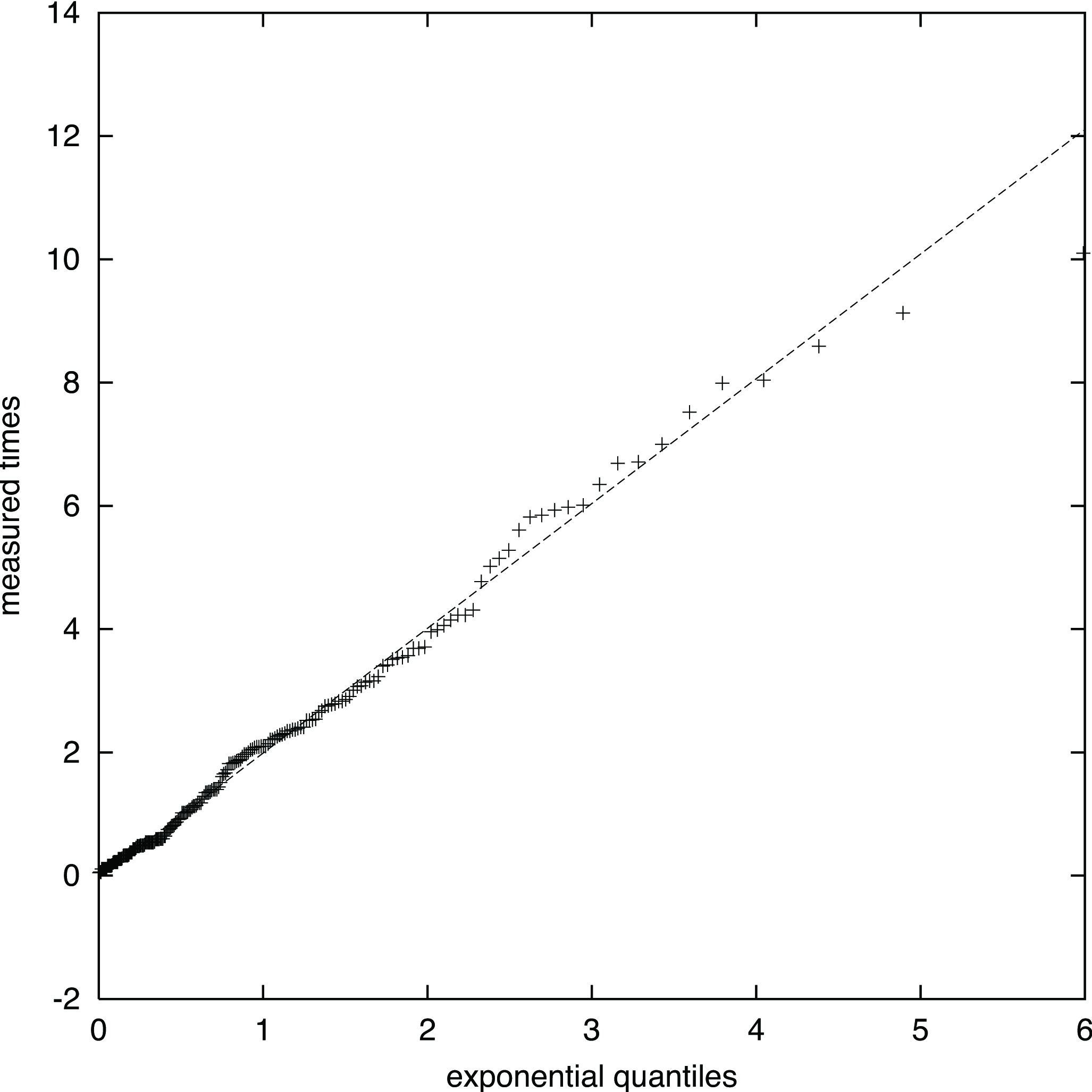
In a situation where the theoretical distribution is a close approximation of the empirical distribution, the points in the Q-Q plot will have a nearly straight configuration. If the parameters L and M of the theoretical distribution that best fits the measured data could be estimated a priori, the points in a Q-Q plot would tend to follow the line x = y. Alternatively, in a plot of the data against a two-parameter exponential distribution with L = 1 and M = 0, the points would tend to follow the line y = L x + M. This means that a single theoretical Q-Q plot compares a set of data not just to one theoretical distribution, but simultaneously to a whole family of distributions. Consequently, parameters L and M of the two-parameter exponential distribution can be estimated, respectively, by the slope L and intercept M of the line depicted in the Q-Q plot.


Q-Q plot
Figure 2 - Q-Q plot


The Q-Q plot shown in Figure 2 is obtained by plotting the measured times in the ordinate against the quantiles of a two-parameter exponential distribution with L = 1 and M = 0 in the abscissa, given by -ln(1-p(i)) for i = 1, ...,n. To avoid possible distortions caused by outliers, we do not estimate the distribution mean with the data mean or by linear regression on the points of the Q-Q plot. Instead, we estimate the slope L of line y = L x + M using the upper quartile q(u) and lower quartile q(l)  of the data. The upper and lower quartiles are, respectively, the Q(1/4) and Q(3/4) quantiles. We take L = [z(u) - z(l)]/[q(u) - q(l)] as an estimate of the slope, where z(u) and z(l) are the u-th and l-th points of the ordered measured times, respectively. This informal estimation of the distribution of the measured data mean is robust since it will not be distorted by a few outliers (Chambers et al., 1983).

To analyze the straightness of the Q-Q plots, we superimpose them with variability information. For each plotted point, we show plus and minus one standard deviation in the vertical direction from the line fitted to the plot. An estimate of the standard deviation for point z(i), i = 1, ...,n, of the Q-Q plot is
s = L [p(i)/(1- p(i))n]˝.


QQ-plot with variability information
Figure 3 - Example of a Q-Q plot with superimposed variability information.


Figure 3 shows an example of a Q-Q plot with superimposed variability information.

When observing a theoretical quantile-quantile plot with superimposed standard deviation information, one should avoid turning such information into a formal test. One important fact that must be kept in mind is that the natural variability of the data generates departures from the straightness, even if the model of the distribution is valid. The most important reason for portraying standard deviation is that it gives us a sense of the relative variability of the points in the different regions of the plot. However, since one is trying to make simultaneous inferences from many individual inferences, it is difficult to use standard deviations to judge departures from the reference distribution. For example, the probability that a particular point deviates from the reference line by more than two standard deviations is small. But the probability that at least one of the data points deviates from the line by two standard deviations is probably much greater. In order statistics, this is made more difficult by the high correlation that exists between neighboring points. If one plotted point deviates by more than one standard deviation, there is a good chance that a whole bunch of them will too. Another point to keep in mind is that standard deviations vary substantially in the Q-Q plot, as can be observed in the Q-Q plot in Figure 4 that the standard deviations of the points near the high end are substantially larger then the standard deviation of the other end.

Empirical and theoretical distributions
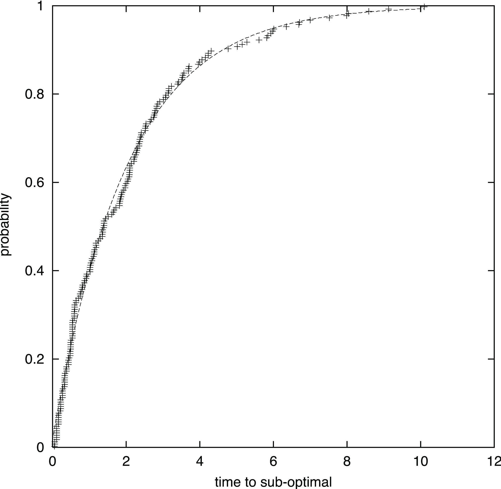
Figure 4 - Superimposed plot of the empirical and theoretical distributions.


Once the two parameters of the distribution are estimated, a superimposed plot of the empirical and theoretical distributions can be made. Figure 4 shows this plot corresponding to the Q-Q plot in Figure 3.


TTTPLOTS.PL - A PERL PROGRAM TO PRODUCE TTT PLOTS

tttplots.pl is a perl program that takes as input a file with n lines, each with one CPU time entry, and produces two plots: 1) superimposed empirical and theoretical distributions; 2) Q-Q plot with superimposed variability information.  In addition to the plots, several output files are also generated.

To download tttplots.pl click here.

To run tttplots.pl, simple type:

         perl tttplots.pl -f input_filename

where input_filename.dat is the input data file with n CPU time data points, one per line.

Besides printing to the standard output some basic statistics about the data file and the estimated parameters, the following output files are produced by tttplots.pl:

empirical exponential distribution data file
input_filename-ee.dat
theoretical exponential distribution data file  input_filename-te.dat
empirical QQ-plot data file
input_filename-el.dat
theoretical QQ-plot data file
input_filename-tl.dat
theoretical upper 1 standard deviation QQ-plot data
input_filename-ul.dat
theoretical lower 1 standard deviation QQ-plot data input_filename-ll.dat
theoretical vs empirical TTT plot gnuplot file
input_filename-exp.gpl
theoretical vs empirical QQ-plot gnuplot file
input_filename-qq.gpl
theoretical vs empirical TTT plot PostScript file
input_filename-exp.ps
theoretical vs empirical QQ-plot PostScript file
input_filename-qq.ps


NOTE:  tttplots.pl requires that gnuplot be installed on system.


REFERENCES

R.M. Aiex, M.G.C. Resende, and C.C. Ribeiro, Probability distribution of solution time in GRASP: An experimental investigation, J. of Heuristics, vol. 8, pp. 343-373, 2002.

R. Battiti and G. Tecchiolli. Parallel biased search for combinatorial optimization: Genetic algorithms and TABU. Microprocessors and Microsystems, 16:351-367, 1992.

J. M. Chambers, W. S. Cleveland, B. Kleiner, and P. A. Tukey. Graphical Methods for Data Analysis. Chapman & Hall, 1983.

N. Dodd. Slow annealing versus multiple fast annealing runs: An empirical investigation. Parallel Computing, 16:269-272, 1990.

H.M.M. Ten Eikelder, M.G.A. Verhoeven, T.W.M. Vossen, and E.H.L. Aarts. A probabilistic analysis of local search. In I.H. Osman and J.P. Kelly, editors, Metaheuristics: Theory & applications, pages 605-618. Kluwer Academic Publishers, 1996.

L.J. Osborne and B.E. Gillett. A comparison of two simulated annealing algorithms applied to the directed Steiner problem on networks. ORSA J. on Computing, 3:213-225, 1991.

B. Selman, H.A. Kautz, and B. Cohen. Noise strategies for improving local search. In Proceedings of the AAAI-94, pages 337-343. MIT Press, 1994.

E.D. Taillard. Robust taboo search for the quadratic assignment problem. Parallel Computing, 17:443-455, 1991.

M.G.A. Verhoeven and E.H.L. Aarts. Parallel local search. J. of Heuristics, 1:43-66, 1995.